As a R learner programmer, it took me unconscionably long to work out how to use polygon to shade under and between curves, despite searches of the R manual and R-help – they just didn’t start far enough back. So, for anyone else scratching his or her head over polygon (and so I can find it again when I forget how it’s done), here are the series of steps I went through to figure it out.
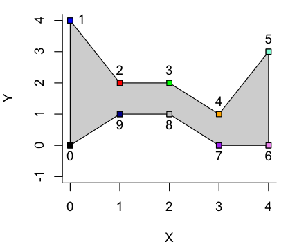
The function takes in an x vector and a y vector, defining a set of coordinates that, in order, taken in order trace around the area to be shaded. Thus for a set of points 1-10, defined individually as x.1, y.1 to x.10, y.10,
x <- c(x.1,x.2,x.3,x.4,x.5,x.6,x.7,x.8,x.9,x.10)

y <- c(y.1,y.2,y.3,y.4,y.5,y.6,y.7,y.8,x.9,y.10)
The area inside these points is shaded by
polygon(x,y,col=gray(0.8))
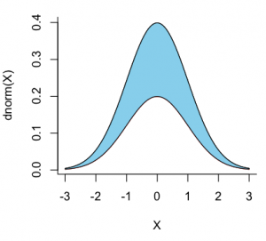 To apply this to two curves, both normal distributions between -3 and 3, one half the height of the other
x <- seq(-3,3,0.01)

y1 <- dnorm(x,0,1)

y2 <- 0.5*dnorm(x,0,1)

plot(x,y1,type="l",bty="L",xlab="X",ylab="dnorm(X)")

points(x,y2,type="l",col="red")

polygon(c(x,rev(x)),c(y2,rev(y1)),col="skyblue")
The first half of the x-vector in the polygon is just the values of x itself, corresponding to the part of the polygon that is tracing out the upper curve along increasing values of x. The second part for of the x-vector in the polygon is the reverse of x, corresponding to the part of the polygon that is tracing out the lower curve along decreasing values of x. The first part of the y-vector is the y values of the upper curve, and the second part of the y-vector is the y values of the lower part of the curve.
That shaded the area between the curves along the full plotted range.
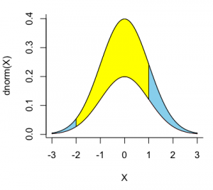 To shade only a defined portion, say the area from x=-2 to x=1.
x <- seq(-3,3,0.01)

y1 <- dnorm(x,0,1)

y2 <- 0.5*dnorm(x,0,1)

x.shade <- seq(-2,1,0.01)

polygon(c(x.shade,rev(x.shade)),c(dnorm(x.shade,0,1),0.5*dnorm(rev(x.shade),0,1)),col="yellow")
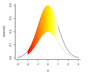 To shade the same defined portion as a gradient, from red to yellow (from the built-in heat.colors palette):
x <- seq(-3,3,0.01)

y1 <- dnorm(x,0,1)

y2 <- 0.5*dnorm(x,0,1)

x.shade <- seq(-2,1,0.01)

par(oma=c(1,1,1,1),cex=0.7)

plot(x,y1,type="l",bty="L",xlab="X",ylab="dnorm(X)")

points(x,y2,type="l",col="gray")

l <- length(x.shade)

color <- heat.colors(l)

for (i in 1:l)

{

polygon(c(x.shade[i],rev(x.shade[i])),c(dnorm(x.shade[i],0,1),

0.5*dnorm(rev(x.shade[i]),0,1)),border=color[i],col=NA)

}
This draws a succession of individual polygons between the curves, adjusting the color along the gradient as it goes. (Note that the loop above is for i in one to letter-L).
